SQL Queries Explained: A Simple Guide to Queries and Databases

Today, data is the engine driving our modern world. To put things in perspective, we generated a mind-boggling 120 zettabytes of data in 2023 alone, that’s roughly 130.9 quadrillion gigabytes! This massive wave of information tracks everything from our favorite streaming shows and online bank transfers to global shipping and healthcare records. To make sense of this endless sea of information, developers rely on powerful tools called Database Management Systems (DBMS) to keep everything organized and accessible.

Picking the right database is crucial for any app’s speed and reliability. While newer “NoSQL” databases are great for flexible, less organized information, like Amazon user reviews, traditional Relational Databases are still the undisputed kings of highly structured data. Think of retail giants like Walmart: they need absolute, foolproof accuracy for their global inventory and financial records, so they rely on the strict rules of relational databases to ensure no items or dollars are ever lost in the system. Within this highly organized world, MySQL remains one of the most popular and widely used options on the planet.

The initial conceptual challenge that a developer faces when entering this ecosystem is why a relational database is required, as compared to a simple and familiar tool such as a two-dimensional spreadsheet. When a small business tries to organize its business operations, customers, products and sales tracking on one large spreadsheet, it is bound to run into extreme structural failures referred to as modification anomalies. Since the spreadsheet requires duplicating the information, it is possible that re-entry of the address of one customer to ship them will necessitate the manual modification of dozens of rows. When one row is ignored, the data will be inconsistent in nature. To add to this, deletion anomalies do exist; since a business deletes every purchase record of a given discontinued item, there exists the possibility of a deletion accident of a customer who had purchased the given item.

Relational databases resolve these anomalies through a mathematical process known as normalization. Normalization dictates that data must be divided into single-themed, discrete tables, eliminating redundant information. To navigate and manipulate this fragmented but highly organized data, developers utilize Structured Query Language (SQL).

Think of a MySQL database as a giant commercial warehouse. The database is a specific room, and the “tables” are organized storage shelves holding your actual items (the data). MySQL acts as the warehouse manager who does all the heavy lifting to store and retrieve those boxes. As the developer (the warehouse owner), you can’t just walk in and move things around yourself. Instead, you have to ask the manager to do it for you using a very specific set of instructions. That language is SQL.

Because SQL is a formal programming language, there is no room for ambiguity or conversational interpretation. In an informal language like English, humans use context to determine what a speaker means. Still, in a formal language like SQL, the database engine executes exactly what is written, regardless of the developer’s intent. Therefore, mastering the precise syntax and underlying logic of MySQL queries is an absolute necessity for any software developer.

Data Definition Language (DDL): Constructing the Foundation

Before any data can be stored, queried, or manipulated, the structural containers for that data must be meticulously defined. This architectural phase is executed using a subset of SQL known as Data Definition Language (DDL). These commands communicate directly with the MySQL engine to create, alter, or permanently destroy structural elements within the database environment.

Establishing the Database Schema

The initialization of any new software project begins with the creation of the database itself. The command CREATE DATABASE database_name; instructs the MySQL engine to allocate a new logical space on the server. Once this space is created, the developer must explicitly instruct the engine to operate within this specific environment using the USE database_name command. Returning to the warehouse analogy, this is the equivalent of the manager unlocking and stepping into a specific room before beginning to construct the storage shelves.

To understand the practical application of DDL commands, one must examine a consistent, real-world database schema. A schema is not merely a visual diagram; it is the collection of coded rules and relationships that define the data’s structure within the database engine. A standard educational model is a centralized Bookstore Management System. A robust bookstore schema requires discrete tables to represent distinct entities: the books themselves, the registered customers, the historical orders, and the marketing expenditures used to acquire those customers.

Creating these individual tables involves the CREATE TABLE statement, which explicitly defines the table name, the required columns, their specific data types, and any enforced constraints.

SQL DDL Command	Functional Purpose	Syntactical Example
SHOW DATABASES;	Queries the server to list all currently available databases.	SHOW DATABASES;
CREATE DATABASE	Initializes a completely new database environment.	CREATE DATABASE Bookstore;
USE	Sets a specific database as the active target for subsequent operations.	USE Bookstore;
CREATE TABLE	Defines a new table schema, including columns and data types.	CREATE TABLE Books (id INT, title VARCHAR(255));
SHOW TABLES;	Lists all tables contained within the currently active database.	SHOW TABLES;
DESCRIBE	Displays the internal schema, column names, and data types of a table.	DESCRIBE Books;
ALTER TABLE	Modifies an existing table’s structure, such as appending a new column.	ALTER TABLE Books ADD price DECIMAL(7,2);
DROP TABLE	Permanently and irreversibly deletes a table and all its contained data.	DROP TABLE Old_Inventory;

The Critical Nature of Data Types

When setting up a new table, you have to tell the database exactly what kind of information belongs in each column. This helps the system save storage space and handle the data correctly, like knowing when it needs to do math or sort by date. For example, text is usually categorized as VARCHAR (perfect for short things like names or emails) or TEXT (better for long paragraphs like a book summary).

Numbers need careful sorting, too. Use INT for whole numbers, like inventory counts. For money, always use DECIMAL (like DECIMAL(7,2), which allows 7 total digits, including 2 for cents) so you don’t lose pennies to rounding errors! Finally, always save dates as DATE or DATETIME. A huge beginner mistake is saving dates as plain text. If you do, the database won’t know how to sort them from oldest to newest without slowing down your whole system.

Primary and Foreign Keys

The true computational superiority of a relational database lies in the prefix “relational.” The single-themed tables generated through normalization do not exist in an isolated vacuum; they are intricately and permanently linked. These critical linkages are established and enforced mathematically through the utilization of Primary Keys and Foreign Keys, which form the absolute bedrock of relational database schema design.

The Primary Key Constraint

A Primary Key is simply a unique ID for every single row in your table. Think of it like a person’s National ID number or a car’s VIN; it guarantees that the database never confuses one record with another. There are only two unbreakable rules for a Primary Key: every ID must be 100% unique, and it can never be left blank (which developers call “NULL”).

In the conceptual Bookstore database, the Books table would assign a unique, numerical book_id to every published title in the inventory. In contrast, the Customers table would assign a unique customer_id to every registered individual. If a primary key is not explicitly defined during the DDL phase, the database engine fundamentally struggles to differentiate between identical records, leading to catastrophic data corruption during modification operations.

To streamline data entry, it is a universal best practice among developers to pair the primary key with an AUTO_INCREMENT attribute. This configuration relieves the application from the burden of generating unique identifiers; whenever a new row is inserted into the table, the MySQL engine automatically calculates and assigns the next available sequential integer. Furthermore, when a primary key is declared, the database engine automatically generates a clustered index for that column behind the scenes, ensuring that retrieving a specific record by its primary key is instantaneously fast.

The Foreign Key and Referential Integrity

While a Primary Key gives a record its own unique ID, a Foreign Key is how different tables connect to each other. It is simply a column in one table that points directly to the Primary Key of another table. This creates a strict, unbreakable link between them, ensuring your database doesn’t end up with messy or orphaned data, like a pending order that belongs to a customer who doesn’t even exist!

A highly illustrative analogy for comprehending foreign keys is the biological parent-child relationship. A single parent entity can have multiple children, but a child entity can only originate from one specific set of parents. In a relational database context, the table containing the original primary key is classified as the “parent” table, and the table containing the referencing foreign key is classified as the “child” table.

Consider the Orders table within the Bookstore schema. An order is not an independent, self-sustaining entity; a specific customer must place it, and it must contain a specific book. Therefore, the Orders table will feature its own primary key (order_id) to uniquely identify the transaction, but it will also contain a customer_id column and a book_id column. These latter two columns are configured as foreign keys.

By defining these columns as foreign keys, the developer instructs the database engine to enforce strict mathematical rules, known as foreign key constraints. The engine acts as a relentless gatekeeper, physically preventing the insertion of an order record if the customer_id provided does not already exist as a primary key in the parent Customers table. This ensures that the system can never process a ghost order for a nonexistent customer.

Furthermore, foreign key constraints govern the database’s behavior when parent records are modified or deleted. Developers can specify actions such as ON DELETE CASCADE within the table definition. This command dictates that if a parent record is deleted (for example, a customer deletes their account), the database engine will automatically hunt down and delete all associated child records (all historical orders belonging to that customer) to prevent orphaned data fragments. Alternatively, the RESTRICT constraint operates defensively; it actively prevents the deletion of a parent record if any child records currently depend on it, forcing the developer to address the active orders before removing the customer profile.

Data Manipulation Language (DML)

Once the skeletal structure of the database has been solidified through DDL and secured by primary and foreign keys, the developer transitions to utilizing Data Manipulation Language (DML) to populate the tables with actual information and alter the state of that data over time.

The Insertion of Records

The INSERT INTO statement is the primary mechanism utilized to append new rows of data into an existing table. The formal syntax requires the developer to explicitly specify the target table’s name, the specific columns slated for population, and the corresponding sequential values.

For example, to register a newly acquired customer within the bookstore database, the query must dictate the target columns and provide the exact literal values: INSERT INTO Customers (name, city, signup_date) VALUES (‘Alice’, ‘New York’, ‘2023-01-10’);. Because the customer_id primary key is configured with the AUTO_INCREMENT property, it is deliberately omitted from the INSERT query; the MySQL engine seamlessly intercepts the insertion and assigns the next available sequential identifier. Developers can also execute bulk operations by appending multiple comma-separated sets of values within a single INSERT statement, drastically reducing network round-trips and improving application throughput.

Updating and Deleting Data

As software applications operate over extended periods, data is inherently mutable. Customers relocate to new cities, and the retail prices of books fluctuate based on supply and demand. The UPDATE statement grants developers the ability to modify existing, pre-recorded rows. Conversely, the DELETE statement permanently purges records from a table’s storage.

However, these specific DML operations represent one of the most critical danger zones for novice database developers. A common, notoriously catastrophic mistake across the industry is executing an UPDATE or DELETE statement without tethering it to a WHERE clause.

The WHERE clause is your safety net, it acts as a highly specific filter. If you want to change the price of just one specific book, you have to pinpoint it using its unique ID (for example, WHERE book_id = 4).

But here is the terrifying part: if you forget to include that WHERE clause, the database won’t double-check with you or throw an error. It will take you literally and assume you meant to apply that price change to every single book in your store! Forgetting this one little word can instantly overwrite your entire inventory.

To prevent mistakes when making multiple updates at once, developers use Transactions. Think of a transaction as an “all-or-nothing” safety feature that bundles several steps together.

Imagine transferring money: you withdraw from one account and deposit into another. If the deposit fails for any reason, the database automatically hits the “undo” button on the withdrawal, putting everything back exactly how it was before you started.

This guarantees your system never gets stuck with missing money or half-finished data.

The SELECT Statement

Setting up your database and updating records are important first steps. However, once a database is up and running, developers spend most of their time just searching for information that is already there. To find and pull out exactly what you need, you will rely almost entirely on one powerful command: the SELECT statement.

The fundamental syntax of a retrieval query is conceptually simple but structurally rigid. The developer must logically define what specific columns to retrieve (SELECT), which table to pull the data from (FROM), how to filter the resulting rows (WHERE), how to sort the final output (ORDER BY), and how many results the engine is permitted to return (LIMIT).

DQL Clause	Analytical Functionality	Syntactical Example Context
SELECT	Determines the precise columns that will be projected into the final result set.	SELECT name, city
FROM	Identifies the specific source table housing the target data.	FROM Customers
WHERE	Filters the table rows based on specified logical conditions.	WHERE city = ‘New York’
ORDER BY	Sorts the filtered result set chronologically or alphabetically.	ORDER BY signup_date DESC
LIMIT	Restricts the absolute maximum number of rows returned by the database engine.	LIMIT 10

Advanced Filtering Mechanisms

The WHERE clause serves as the primary mechanism for isolating relevant data, relying on a variety of logical operators to evaluate each row. Developers utilize standard comparative mathematical operators such as =, > , <, and <> (the SQL representation of “not equal to”).

Furthermore, SQL provides advanced operators that allow for highly nuanced data filtering. The IN operator allows a query to match a column’s value against a specified, comma-separated list of potential values, eliminating the need to write endless chains of OR statements. The BETWEEN operator is highly optimized for filtering data that falls within a specific numerical or chronological range, such as locating all orders placed within a specific fiscal quarter.

When precise values are unknown, developers employ pattern matching using the LIKE operator, combined with specialized wildcard characters. The percentage symbol (%) represents zero, one, or multiple unknown characters. For instance, a database query structured as WHERE title LIKE ‘%SQL%‘ will thoroughly scan the table and return any book title containing the acronym SQL, regardless of whether it appears at the beginning, middle, or end of the text string.

The Logical Order of Query Execution

A profound conceptual hurdle for developers transitioning into database engineering is understanding that the syntactical order in which a SQL query is written on the screen is entirely disconnected from the logical order in which the database engine actually executes the operations.

The visual syntax places the SELECT keyword at the very beginning of the written query. However, logically, the database engine cannot select columns from data it has not yet located or filtered. The strict order of execution dictates that the engine first accesses the data source designated in the FROM clause (and executes any table joins). Next, it applies the logical conditions of the WHERE clause, filtering the massive dataset down to the relevant rows. Only after the data has been securely narrowed down does the engine apply any grouping or mathematical aggregations.

Following aggregation, the HAVING clause filters the newly grouped data. Finally, deep into the execution process, the SELECT clause operates. It functions essentially as a projection lens, dictating which specific columns of the heavily filtered and processed data will be made visible in the final output matrix. Once the columns are selected, the resulting dataset is sorted by the ORDER BY clause and truncated by the LIMIT clause. Internalizing this underlying execution pathway is an absolute necessity for writing highly efficient queries and diagnosing complex semantic logic errors.

Aggregate Functions and Data Grouping

While retrieving raw, literal data is a foundational requirement, the true analytical prowess of the MySQL engine emerges through its capacity to instantaneously summarize massive, millions-row datasets into concise, actionable business intelligence metrics. This sophisticated summarization is achieved using Aggregate Functions. An aggregate function performs a mathematical operation across an entire set of rows within a single specified column, collapsing the data down to return a single, calculated value.

Core Aggregate Functions

The most frequently deployed aggregate functions form the backbone of modern data analytics and reporting dashboards:

• COUNT(): Calculates the total numerical volume of rows that match the query’s criteria. It is universally used to determine volume metrics, such as calculating the total number of orders placed in a given month (SELECT COUNT(*) FROM Orders;).
• SUM(): Computes the total mathematical addition of a numeric column. This is essential for calculating enterprise-level metrics, such as aggregating total gross revenue or tallying physical inventory counts (SELECT SUM(price) FROM Books;).
• AVG(): Determines the mean average value of a specific numeric column, highly useful for identifying consumer trends, such as the average cart value of an e-commerce platform.
• MIN() and MAX(): Systematically identify the absolute lowest and highest values contained within a column, respectively. These functions are remarkably versatile; they can be applied to numerical financial data, alphabetical textual strings to find the first or last entry, or chronological date columns to easily locate the very first or most recent transaction in a company’s history.

The Conceptual Mechanics of the GROUP BY Clause

Math functions like SUM become a lot more useful when you team them up with the GROUP BY command. Adding up the value of every book in your entire store is okay, but you usually want more specific answers, like the total value of books organized by genre. The GROUP BY clause simply tells the database to sort your items into distinct piles first (like separating Sci-Fi from Romance), and then do the math for each pile separately.

A highly illustrative, non-technical metaphor for comprehending the GROUP BY operation is the domestic chore of doing laundry. If an individual simply gathers all their clothing and dumps it into a washing machine simultaneously, the machine processes the load indiscriminately, resulting in a single, undifferentiated output, metaphorically, a single load of pink, ruined laundry. This mirrors the execution of an aggregate function without a GROUP BY clause; the engine processes the entire table as one massive load.

Conversely, if the individual takes the time to systematically sort the laundry into distinct, separate piles, isolating the lights, the darks, and the delicates, and then washes each specific pile independently, they are performing a physical GROUP BY operation.

When a query is structured as SELECT genre, SUM(price) FROM Books GROUP BY genre, the MySQL engine scans the specified ‘genre’ column, creates a distinct, isolated “pile” in memory for every unique genre it encounters (Fiction, Technology, Fantasy), and then calculates the SUM function independently for each pile.

Post-Aggregation Filtering: The HAVING Clause

One of the biggest mix-ups for developers is knowing when to use WHERE versus HAVING. Both commands actually do the same job, filtering out data you don’t want to see. The tricky part is that they do their filtering at completely different steps in the process.

The WHERE clause operates strictly on individual, raw rows before any grouping or mathematical aggregation takes place. In stark contrast, the HAVING clause was engineered into the SQL language specifically to filter data after it has been grouped and aggregated.

If you want to find book genres with an average price over $20, you can’t use WHERE. Why? Because that “average” doesn’t actually exist in your database yet; it’s a brand new number the system calculates on the fly.

If you try to filter by it using WHERE, you’ll just get an error. Instead, you have to group the books first, calculate the average for each pile, and then filter those new piles using HAVING AVG(price) > 20.

Refining Output: DISTINCT and the Abstract Nature of NULL

As SQL queries scale in complexity, particularly when joining multiple tables together, managing duplicate records and absent data becomes critical for generating mathematically accurate analytics.

The DISTINCT Clause

The DISTINCT command is your tool for cleaning up messy, repetitive lists. If you ask your database for a list of shipping cities, it might spit out “New York” a thousand times if a thousand different orders went there. But by adding the word DISTINCT right after SELECT, the system automatically strips away all those duplicates, handing you a clean, simple list of unique cities.

A highly common and detrimental mistake in data science pipelines is neglecting to apply the DISTINCT keyword when attempting to calculate the volume of unique users interacting with a software system. If a developer uses a simple COUNT(user_id) on an activity log, a single highly active user who logged in fifty times will be counted fifty times, severely inflating and skewing the application’s true engagement metrics.

It is also crucial to conceptually differentiate the DISTINCT query clause, which merely filters the visual output of a specific query, from the UNIQUE table constraint, which is an immutable structural rule applied to a table’s column during the DDL phase to violently reject and prevent duplicate data from ever being written to the disk in the first place.

Comprehending the NULL State

In the database world, NULL is highly misunderstood. It is crucial to remember that NULL does not mean the number zero, and it isn’t just an empty text box. Instead, NULL simply means a total unknown. It is the database’s way of throwing its hands up and saying, “Data is missing,” “I don’t know,” or “This doesn’t apply.”

Because NULL explicitly represents an unknown state, it cannot be evaluated using standard mathematical equality operators. A SQL query asking WHERE phone_number = NULL will silently fail to return any matching records, because an unknown, abstract value cannot logically equal another unknown value.

Instead, the SQL language mandates that developers use the specialized identity operators IS NULL or IS NOT NULL to specifically interrogate the column for the absence of data.

Furthermore, when the DISTINCT filtering clause encounters multiple rows containing a NULL state in the queried column, the database engine treats all instances of NULL as a single, identical concept, returning only one representation of NULL in the final deduplicated output matrix.

Demystifying SQL JOIN Operations

Relational databases deliberately store related information in separate, highly normalized tables to preserve referential integrity and brutally eliminate data redundancy.

However, software applications and reporting dashboards rarely require data in total isolation. To present a unified, cohesive view to the end-user, the database engine must dynamically reconstruct these severed relationships on the fly. This massive computational operation is executed using the JOIN clause, universally considered the most critical, powerful, and nuanced conceptual hurdle in SQL mastery.

A JOIN operation essentially functions as a directive to the MySQL engine, instructing it to stitch together discrete rows from two or more independent tables based on a shared, related column.

In properly designed schemas, this connection is almost exclusively established between the primary key of the parent table and the foreign key of the child table.

Visualizing the Mechanics of Joins

The pedagogical challenge of explaining joins often relies heavily on visual analogies. The most ubiquitous visualization tool in the industry is the mathematical Venn diagram, which represents sets of data overlapping and intersecting in circles.

While a Venn diagram is arguably useful for giving absolute beginners a cursory visualization of the final data output (e.g., the overlapping center of the circles represents matching records), senior database architects argue that Venn diagrams fail catastrophically to accurately depict the internal, mechanical actions of how the database engine actually combines the rows.

Venn diagrams completely break down conceptually when multiple matching rows exist, which leads to multiplication of data, or Cartesian products, a reality that set-theory circles cannot visually accommodate.

A vastly more robust and mechanically accurate analogy is a complex social mixer taking place in the lobby of a large apartment building. Imagine two distinct groups of individuals attending the event.

The first group consists of registered tenants who lease apartments in the building (Table A). The second group consists of individuals carrying pets (Table B). Naturally, some tenants own pets, some tenants do not own pets, and some pet owners attending the mixer are visiting guests who do not live in the building.

A database join operation is the systematic process of the database engine walking through the room and attempting to pair people up based on a highly specific, shared characteristic, for instance, their exact Social Security Number.

If Table A (Orders) contains a list of financial purchases with a customer_id attached, but completely lacks the customer’s physical shipping address, and Table B (Customers) contains the physical shipping addresses linked to the same customer_id, the database utilizes a join.

The engine essentially queries the room, asking, “Can we find matching customer_ids in both of these tables simultaneously?” When a perfect match is located, it allows the Order record to borrow the matching Customer address data and merge them into a single row.

A Taxonomy of JOIN Types

The specific type of join declared by the developer dictates exactly how the engine must handle the “leftover” records, the individuals at the social mixer who do not possess a matching partner in the opposing table.

Logical Join Type	Internal Mechanism of Action	Output Behavior and Handling of Unmatched Rows
INNER JOIN	Retrieves exclusively the records that possess mathematically matching values in both tables being joined.	The strictest join. If an Order exists but the associated Customer profile was somehow deleted, the Order is ruthlessly excluded from the final results.
LEFT JOIN (Left Outer Join)	Retrieves all records from the “Left” table (the first table declared sequentially in the FROM clause), along with any matching records from the “Right” table.	The most common outer join. If a Left table row has zero matches in the Right table, the engine returns the Left row anyway, dynamically filling the Right table’s missing columns with NULL values.
RIGHT JOIN (Right Outer Join)	The exact logical inverse of the Left Join. It prioritizes the retrieval of all records from the “Right” table.	Utilized significantly less frequently in production, as almost all queries can simply be restructured as a highly readable Left Join simply by reversing the sequential order of the tables in the syntax.
FULL OUTER JOIN	Combines the comprehensive effects of both Left and Right joins simultaneously, guaranteeing the return of all rows from both tables regardless of whether a matching relationship exists.	Any unmatched rows on either the left or right side are populated entirely with NULL values. (Note: The MySQL engine inherently does not support native FULL OUTER JOIN syntax; developers must simulate it by executing a UNION between a Left Join and a Right Join).
CROSS JOIN	Produces the complete Cartesian product of the two tables, ignoring any shared keys or relationships.	Pair every single row in Table A with every single row in Table B. If Table A contains 100 rows and Table B contains 100 rows, the output is a massive 10,000 rows. Highly dangerous if executed accidentally.
SELF JOIN	A specialized architectural technique where a single table is joined mathematically to itself.	Exceptionally useful for querying hierarchical or nested data, such as an Employees table where a manager is also technically an employee listed in the same table.

Knowing the difference between an INNER JOIN and a LEFT JOIN is a game-changer. Imagine you need to pull a complete list of all your users and their total purchases.

If you use a strict INNER JOIN, the database will silently hide anyone who hasn’t bought something yet, accidentally leaving them off your report!

But if you use a LEFT JOIN, it guarantees that every single user makes it onto the list. The people who haven’t made a purchase yet will simply show up with a blank (or NULL) next to their name.

Database Optimization and Performance Tuning

As a database scales from local development environments containing hundreds of rows to enterprise production environments containing hundreds of millions of rows, the computational and hardware cost of retrieving data increases exponentially.

A poorly structured SQL query that executes instantaneously on a developer’s laptop might take several minutes to process on a production server, locking up hardware resources, severely degrading application performance, and alienating users.

Consequently, mastering fundamental query optimization is absolutely imperative for backend engineering.

The Mechanism of Database Indexes

The single most impactful, paradigm-shifting optimization technique available to a developer is the strategic implementation of database indexes. To fully comprehend the sheer power of an index, one must consider a massive, thousand-page physical textbook completely devoid of a table of contents or an index at the back.

If a reader is tasked with finding every specific mention of the word “algorithm” within the text, they have absolutely no alternative but to start at page one and read every single word sequentially until the end of the book.

In database architecture terminology, this is known as a Full Table Scan. It is a devastatingly resource-intensive operation that forces the physical storage disk to read every single row in the table into memory.

A database index functions identically to the index found at the back of that textbook. It is a completely separate, highly organized internal data structure, almost universally structured mathematically as a B-Tree, that is generated and meticulously maintained by the database engine.

When a developer issues a DDL command to create an index on a specific column, for instance, CREATE INDEX idx_user_id ON users (id);, the engine systematically builds a sorted, easily searchable map of that column’s values.

Each value in this map contains a direct, physical pointer to the exact location of the full row on the server storage disk.

When a subsequent query utilizes that specifically indexed column in its WHERE, JOIN, or ORDER BY clauses, the engine completely bypasses the table data. Instead, it consults the B-Tree index structure, navigates it mathematically in $O(\log n)$ time complexity, pinpoints the exact physical location of the requested data, and retrieves only those specific rows without scanning the remainder of the table.

For queries that routinely filter based on multiple columns simultaneously (e.g., searching for a specific product_id purchased on a specific order_date), developers implement Composite Indexes, which map multiple columns together into a single, highly efficient B-Tree.

However, indexing is a highly delicate architectural balancing act. Every single time a new row of data is inserted, updated, or deleted via a DML command, the database engine must pause to recalculate, re-sort, and rewrite every single index associated with that modified table.

Therefore, while indexes drastically and exponentially accelerate read operations (SELECT), an overabundance of unnecessary or redundant indexes will severely penalize and throttle write operations (INSERT, UPDATE), consuming vast amounts of premium disk storage space and processing CPU overhead.

Eradicating the SELECT * Anti-Pattern

A ubiquitous, deeply entrenched, and highly detrimental habit among novice developers is the liberal use of SELECT * (Select All) in production environments.

While highly convenient for rapid visual debugging in a local console, executing SELECT * from a table within application code forces the database engine to extract and transmit every single column defined in the table, regardless of whether the software application actually requires or consumes that data.

If a web application only needs to display a simple list of user email addresses on a dashboard, retrieving the user’s heavily encrypted password hash, their lengthy biographical text column, and their profile image binary data wastes massive amounts of server RAM, CPU processing cycles, and network bandwidth.

Optimizing this common bottleneck simply involves strictly and explicitly naming the exact required columns in the query: SELECT email FROM users;.

This minor syntactical adjustment reduces disk Input/Output (I/O) and network payload sizes dramatically, freeing up resources for concurrent operations.

Leveraging Query Planners and LIMIT Controls

When constructing highly complex queries involving multiple nested joins, subqueries, and sophisticated filtering conditions, developers cannot rely on guesswork to determine performance. Instead, they must leverage the EXPLAIN statement.

When the EXPLAIN keyword is prepended to any SELECT query (e.g., EXPLAIN SELECT name FROM Customers...), the command issues a directive preventing the query from actually executing against the data.

Instead of returning rows, the database engine returns a Query Execution Plan, a highly detailed, step-by-step blueprint of exactly how its internal optimizer intends to execute the query.

This diagnostic blueprint explicitly reveals whether the engine intends to successfully utilize the B-Tree indexes or if it is being forced to perform catastrophic full table scans.

This allows the database architect to proactively diagnose and rewrite bottlenecks before the flawed code is ever deployed to a production environment.

Furthermore, developers must ruthlessly and systematically utilize the LIMIT clause to constrain data payloads. If a user executes a generic search for a product category, and the database contains 50,000 matches, the application’s user interface fundamentally cannot render 50,000 results simultaneously on the screen.

By appending LIMIT 20 to the query, the database engine is explicitly instructed to immediately halt its disk search and return data the exact millisecond it locates the first 20 valid matches, saving immense computational effort and rendering the application highly responsive.

However, a profound implicit danger lies in deploying LIMIT without an accompanying ORDER BY clause. Because relational database engines inherently do not guarantee any natural or chronological row order on the physical disk, issuing a LIMIT directive without strict sorting parameters will return a completely unpredictable, non-deterministic, and randomized sample of rows every time the query is run, leading to bizarre application behavior.

Hardware and Architectural Considerations

While flawless SQL syntactical proficiency is vital, the underlying physical hardware of the server heavily dictates the maximum theoretical database throughput. The MySQL engine relies massively on RAM (Memory) to temporarily cache frequently accessed data and indexes for instantaneous retrieval.

the InnoDB Buffer Pool is the primary, dedicated memory space where MySQL caches this information.

If a database architect allocates insufficient memory to the Buffer Pool, the engine is forced to constantly dump data from RAM and read it directly from the slow physical disk platter.

This cycle leads to severe I/O bottlenecks, massive latency spikes, and potentially catastrophic “Out of Memory” (OOM) application crashes.

To further alleviate systemic stress on the primary database, senior architects frequently implement Connection Pooling. Rather than forcing the server to spin up a computationally expensive, entirely new network connection for every single incoming user request, Connection Pooling maintains a steady cache of open, ready-to-use connections that the application can briefly borrow and return.

Additionally, in highly scaled environments, read-heavy workloads (like generating analytics reports) are geographically distributed by routing SELECT queries to secondary Read Replicas, thereby preserving the primary database’s processing CPU power exclusively for mission-critical write operations.

Security Posture: Vulnerability Mitigation and Defense

A comprehensive analysis of SQL and relational databases is fundamentally incomplete without aggressively addressing cybersecurity.

Because the database system acts as the centralized repository for an organization’s most sensitive and highly regulated information, ranging from encrypted financial records to proprietary intellectual property and user credentials, it represents the primary, highest-value target for malicious threat actors globally.

The Mechanics of SQL Injection (SQLi)

SQL Injection (SQLi) is the most prevalent, perilous, and the simplest to pull-off web security attack on the Internet today. The catch? A bug or defect in the database software itself does not cause it.

Rather, it occurs when a website has gone wrong and sees regular textual input of a user, such as typing something in a search box or in a login screen, as a real, executable database query.

To understand the exploit, consider a standard web application login form where a user types their username and password.

An insecure, poorly programmed application might take that raw input text and concatenate it directly into a raw SQL command string:

SELECT * FROM users WHERE username = ' + input_user + ' AND password = ' + input_pass + ';

Imagine a hacker types a tricky phrase like ‘ OR ‘1’=’1 into the username box. Because of how the website stitches this text into its database commands, it completely changes the underlying logic.

Instead of securely asking, “Does this exact username and password match?”, the database is tricked into asking, “Does this username match, OR is 1 equal to 1?“

Because the mathematical statement ‘1’=’1′ is an absolute, universally true boolean expression, the entire WHERE clause’s restrictive condition is instantly and irrevocably satisfied for every single row present in the table.

The database engine, behaving exactly as it was formally programmed to do, evaluates the condition as True, entirely bypasses the password authentication check, and grants the attacker unauthorized administrative access to the system.

Successful SQLi exploits provide attackers with unfettered access. Depending on the database permissions, attackers can quietly exfiltrate massive volumes of sensitive customer data (data breach), maliciously alter account balances or permissions, execute complete data deletion, or even issue system-level administrative commands to force a shutdown of the entire DBMS, triggering catastrophic downtime.

Hackers have a few clever ways to sneak these attacks in. The most common method is surprisingly direct: they just use your website’s normal search bars or forms to pull the stolen data right out.

Another trick is purposely typing broken commands to make your database crash. When it crashes, it often spits out detailed error messages meant for developers.

To a hacker, those error messages are like a free blueprint showing them exactly how your database is built so they can plan a bigger attack.

And remember, it doesn’t matter what programming language your site uses; this flaw happens simply when user text isn’t handled securely.

Mitigation via Prepared Statements

The ultimate and uncompromising protection against SQL injection attacks is the complete and utter elimination of the raw and string-concatenated SQL queries in application program code.

In order to accomplish this, developers must shift purely to the use of Prepared Statements (also officially called in the industry as parameterized queries).

The best way to fix this security flaw is by using something called a Prepared Statement. Instead of sending the database the command and the user’s text all mixed at the same time, you split it into two steps.

First, you send the database an empty blueprint or a “fill-in-the-blanks” version of your command, using simple question marks (?) as safe placeholders where the user’s data will eventually go.

SELECT * FROM users WHERE username =? AND password =?;

Upon receiving this blueprint, the MySQL database engine parses, compiles, and locks the structural execution path of the query.

Only after this structure is immutably locked does the application transmit the user’s input parameters to “fill in the blanks”. Because the query’s structural commands are already fully compiled, the database engine treats the subsequent user input strictly as literal, benign textual data and never as executable commands.

Even if a malicious actor inputs destructive SQL syntax like ‘ OR ‘1’=’1, the engine is mathematically incapable of executing it; it will simply, and harmlessly, search the database for a user whose literal, actual username is exactly the string “‘ OR ‘1’=’1″, rendering the SQL injection attempt completely inert and harmless.

Addressing Advanced Pitfalls

Beyond securing the database against external malicious actors, inexperienced developers frequently stumble into advanced semantic errors that do not trigger application crashes or error codes.

Instead, these errors silently return wildly inaccurate data matrices, leading to fundamentally flawed business intelligence and catastrophic decision-making.

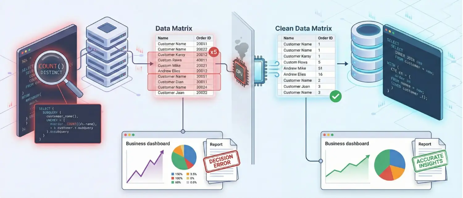
A highly frequent error in data engineering involves a fundamental misunderstanding of how the engine handles data deduplication when executing partial cross joins.

If an analyst attempts to calculate the total number of distinct orders by joining the Customers table to the Orders table, and a single, highly active customer has placed five distinct orders, the resulting mathematical join operation will output five duplicated rows for that specific customer.

If the developer carelessly runs a COUNT() aggregation without the DISTINCT modifier, that single customer is counted five times instead of once, destroying the accuracy of the metric.

Conversely, attempting to mask a poorly constructed, exploding Cartesian join by simply slapping the DISTINCT keyword onto the SELECT clause is widely recognized by senior architects as a severe anti-pattern.

It forces the database engine to waste massive CPU cycles performing unnecessary mathematical pairing and memory allocation before frantically filtering out the millions of duplicate errors it just artificially created.

Finally, the systemic overuse of nested subqueries is a common crutch for developers transitioning into complex data retrieval. While a subquery, a fully independent SQL query nested directly inside a WHERE or FROM clause of a larger query, is perfectly valid syntax, poorly optimized correlated subqueries can be forced by the engine to execute repeatedly for every single row evaluated by the outer, primary query.

In almost all high-performance scenarios, refactoring the nested logic to utilize a standard INNER JOIN or establishing a Common Table Expression (CTE) provides the database optimizer with a vastly more efficient, readable, and performant execution pathway.

About the writer

Hassan Tahir wrote this article, drawing on his experience to clarify WordPress concepts and enhance developer understanding. Through his work, he aims to help both beginners and professionals refine their skills and tackle WordPress projects with greater confidence.