The relational database management system (RDBMS) is the foundation of information technology in the enterprise over a period of almost 50 years. These systems were designed based on the relational model presented by E.F. Codd in 1970. They were designed to manipulate structured data, information that is easily packed into rows and columns, with strict schemas and queryable using a deterministic query language such as SQL. In the paradigm, information is categorical and discrete. When a query is made with the user ID 1024, a particular record is retrieved with absolute accuracy. This model stimulated the development of transaction systems, from banking ledgers to inventory management, in which precision is the most important.
AI data infrastructure
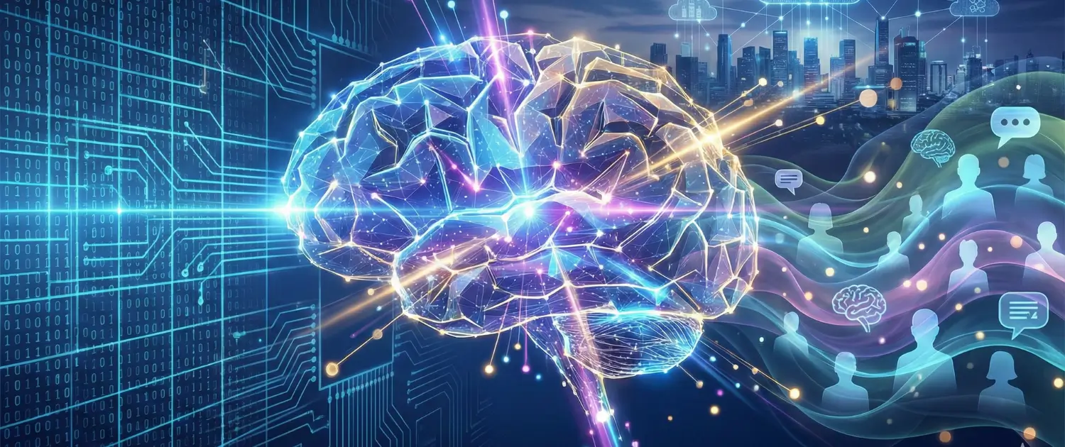
Vector databases power AI search, recommendations, and retrieval workflows. Voxfor VPS gives developers dedicated resources for APIs, dashboards, experiments, and AI-powered applications.
The digital realm has experienced a seismic change. The “Big Data” revolution that was immediately succeeded by the AI revolution has overwhelmed organizations with unstructured data. The unstructured data in the enterprise is estimated to exceed 80 percent (emails, Slack messages, PDF reports, audio recordings, video footage, and social media interactions). This data has no underlying schema. It is disorganized, subtle, and abundant with semantic background, which can not be conveyed by the conventional rows and columns.
The root cause of the failure of traditional databases in this new era is the semantic gap. In a classical database, the string apple and the string i phone are completely different objects unless it is documented that they are connected in any way by a foreign key. It cannot necessarily perceive that the word apple also has anything to do with fruit or pie. Search engines, such as lexical matching techniques (like TF-IDF), were a method used by keyword-based search engines (such as Lucene) to fill this gap by ranking documents by the frequency of occurrence of a word. Lexical search, however, is fragile; it does not support the use of synonyms, polysemy (words with multiple meanings), or intent. When a user types in the word automobile, a keyword engine may not find a relevant document that only contains the word car. The industry needed a system that was able to interpret meaning as opposed to character matching.

Deep learning was the area that provided the solution to the semantic gap, and not database theory. The introduction of Vector Embeddings, mathematical representations of information created by a neural network, has essentially transformed the way machines process information. Embeddings parametrize human-readable information (text, images, audio) into machine-readable vectors: long arrays of floating-point numbers that represent data in a high-dimensional geometrical space.
Semantic meaning is converted to spatial proximity in this high-dimensional space known as a vector space. The main innovation is that the similar concepts are mathematically proximate to each other. King and Queen have a space relationship with each other, just like Man and Woman. Such an innovation has required a new form of database: the Vector Database.
A vector database is not just a storage engine, but a computational engine optimized to carry out the mathematical operations on these high-dimensional vectors at large scale,4 unlike a relational database that is optimized to perform Exact Match (finding the row where x = y) operations. The deterministic to probabilistic retrieval is the keystone to contemporary Artificial Intelligence, as it allows systems to retrieve information based on conceptual relevance, and not on the overlap of keywords.
The vector database has therefore become the long-term memory of the Artificial Intelligence. Similarly to how the human brain uses the hippocampus to retrieve the memories, the vector database uses semantic concepts to index and retrieve them, like the hippocampus does to retrieve human brain memories.<|human|> Similarly to how the human brain uses the hippocampus to retrieve the memories, the vector database uses semantic concepts to index and retrieve them, similar to the hippocampus does to retrieve human memory of the brain.
The first thing to realize when we do not know the mechanism of a vector database is to comprehend the mathematical concepts on which the data it contains is based. The atomic unit of modern AI is the so-called vector, which is the way to transform raw unstructured data into computational understanding.
A vector embedding is an ordered list of numbers (scalars), typically 32-bit floating-point values, which represent the features of a data object.
$$v = [0.12, -0.98, 0.05, 1.23, \dots, n]$$
The length of this list is the dimensionality of the embedding. While a point on a piece of paper has two dimensions (x, y) and a point in physical space has three (x, y, z), vector embeddings in production AI systems often have hundreds or thousands of dimensions. For instance, the popular OpenAI text-embedding-3-small model produces vectors with 1,536 dimensions.
Each dimension in a vector effectively represents a “feature” or characteristic of the data. However, these features are often abstract and learned by the neural network rather than explicitly defined by humans.
The embedding model, a deep neural network like BERT, ResNet, or a Transformer, acts as a complex function $f(x)$ that maps the input $x$ (text/image) to the vector $v$. This process is described as “alchemy” because it distills the messy, unstructured essence of the input into a precise numerical format. The resulting vector sits in a “latent space” or “manifold” where the geometry of the space dictates meaning.
The defining property of this vector space is that distance equals dissimilarity. Items that are semantically related form clusters. In a vector space representing animals:
This clustering allows for powerful operations. We can perform algebra on concepts. The classic example from Word2Vec demonstrates this:
$$\vec{King} – \vec{Man} + \vec{Woman} \approx \vec{Queen}$$
By subtracting the “Man” feature vector from “King” and adding the “Woman” feature vector, the result moves through the vector space to arrive at the coordinates for “Queen“.
To quantify “closeness,” vector databases employ specific mathematical distance metrics. The choice of metric often depends on how the embedding model was trained and the specific nature of the data.
| Metric | Mathematical Concept | Best Application | Nuance |
| Cosine Similarity | Measures the cosine of the angle between two vectors. $Similarity = \frac{A \cdot B}{\|A\| \|$ | Text Analysis, Document Retrieval, NLP | Focuses on the orientation of the vectors rather than their magnitude. Two documents can be similar in topic even if one is much longer (larger magnitude) than the other. This makes it ideal for “flavor profile” matching in text.13 |
| Euclidean Distance (L2) | Measures the straight-line distance between two points. $d(p,q) = \sqrt{\sum (p_i – q_i)^2}$ | Computer Vision, Spatial Data | Sensitive to vector magnitude. Often used when the “intensity” of a feature matters. If vectors are normalized (length = 1), Euclidean distance and Cosine similarity are functionally equivalent.6 |
| Dot Product | The sum of the products of corresponding entries. $A \cdot B = \sum A_i B_i$ | Recommendation Systems, Matrix Factorization | computationally cheaper than Cosine. Highly effective for ranking tasks where magnitude (e.g., popularity or rating strength) is significant. Requires normalized vectors to be a strict similarity measure.13 |
| Manhattan Distance (L1) | The sum of absolute differences. $d(p,q) = \sum | p_i – q_i | $ |
| Hamming Distance | Number of positions at which symbols differ. | Binary Vectors, Hashing | Used for binary embeddings or hash codes, extremely fast but less precise for continuous semantic nuances.13 |
The selection of the correct distance metric is critical. Using Euclidean distance on embeddings trained for Cosine similarity can lead to suboptimal retrieval results, as the geometry of the latent space may be distorted relative to the query mechanism.

While generating embeddings is a function of machine learning models, managing them is a systems engineering challenge. A vector database must store millions or billions of these vectors and retrieve the “Top-K” nearest neighbors to a query vector in milliseconds. This requirement presents a massive computational hurdle known as the Nearest Neighbor Search (NNS) problem.
A small dataset can be searched using a “Flat” / “Brute Force” search: the query vector is compared to each of the individual database vectors, the distance is calculated, and the results are sorted.
Nevertheless, it is not cheaper than $O(N D N), where N and D are the number of vectors and the dimension, respectively. Having 100 million vectors of 1,536 dimensions, one query would take approximately 150 billion floating-point calculations. This is too slow to allow real-time applications. Moreover, the higher the dimension, the higher the volume of the space; therefore, the data are sparse, a phenomenon referred to as the Curse of Dimensionality. The traditional indexing organization, such as B-Trees or KD-Trees, cannot work in high dimensions due to the inefficiency of the branching factor; the algorithm effectively searches most of the branches.
To overcome this, vector databases utilize Approximate Nearest Neighbor (ANN) algorithms. These algorithms trade a negligible amount of accuracy (e.g., finding the true nearest neighbor 99% of the time instead of 100%) for massive gains in speed.
The index is the main element that classifies vectors so that they can be traversed quickly. The modern world of vector databases is dominated by a number of classes of indexing algorithms.
HNSW is currently the industry standard for in-memory vector indexing due to its superior balance of speed and recall.
IVF strategies are based on clustering and are often used when memory is constrained or the dataset is too large to fit entirely in RAM.
With very large datasets that may be larger than available RAM, algorithms such as Vamana (in DiskANN) are implemented such that the majority of the vector data is stored on NVMe SSDs, and a compressed version is held in memory. It enables one machine to process billions of vectors per second (significantly lowering hardware expenses than RAM-only systems such as HNSW).
To further optimize performance and storage, vector databases employ quantization, reducing the precision of the numbers in the vector.
Scalar Quantization converts the floating-point numbers (usually 4 bytes / 32 bits) into smaller integers (e.g., 1 byte / 8 bits).
Product Quantization is a more aggressive compression technique.
While CPUs are sufficient for many workloads, the parallel nature of vector calculations makes them ideal for GPUs (Graphics Processing Units).
The meteoric rise of vector databases in 2023-2024 is inextricably linked to the popularity of Generative AI and Large Language Models (LLMs). While LLMs like GPT-4 are powerful reasoning engines, they suffer from critical “cognitive” limitations that vector databases solve via a pattern known as Retrieval-Augmented Generation (RAG).
LLMs are trained on a massive corpus of public data, but once training is complete, their knowledge is frozen.
RAG architecture decouples “reasoning” (the LLM) from “memory” (the Vector Database). It allows the LLM to access external data dynamically.
The process begins with Data Ingestion. Documents (PDFs, HTML, Text) are collected and split into smaller segments called “chunks”.
When a user asks a question (e.g., “What is the company policy on remote work?”):
The retrieved text chunks are combined into a prompt sent to the LLM:
“Context: [Chunk 1 text][Chunk 2 text]…
User Question: What is the company policy on remote work?
Instruction: Answer the question using ONLY the provided context.”
The LLM generates the answer. By grounding the generation in retrieved facts, hallucinations are drastically reduced, and the model can answer using up-to-the-minute private data.
As RAG moves from prototype to production, simple “retrieve and generate” loops are often insufficient. Advanced patterns have emerged to handle complexity.
While vector search is powerful, it lacks precision for keyword-specific queries. If a user searches for a specific part number “AX-9901“, vector search might return “AX-9902” because they are semantically similar (both part numbers).
Vector search flattens data into a list of isolated chunks, losing the structural relationships between them.
We are currently witnessing a shift from passive “Chatbots” (which respond to user inputs) to active AI Agents (which pursue goals autonomously). Vector databases are evolving to become the Long-Term Memory for these agents.
Standard LLMs are stateless; they reset after every interaction. For an agent to function over days or weeks (e.g., a coding agent building a website), it needs to remember:
Agents utilize vector databases to store these memories.
This persistent state allows for the creation of “Personalized Agents” that adapt to their users’ styles and preferences over long periods, creating a continuous thread of continuity that was previously impossible.
The “Vector” abstraction is universal. It applies not just to text, but to any data type that can be passed through a neural network. This has given rise to Multimodal Vector Search, where images, audio, and video co-exist in the same information space.
Models like CLIP (Contrastive Language-Image Pre-training) or Amazon’s Nova Multimodal Embeddings map different modalities into a shared vector space.
The application of vector databases extends far beyond simple chat applications. They are solving fundamental problems in science, security, and commerce.
Biology is fundamentally a high-dimensional problem.
Cyber threats are constantly evolving, making rule-based detection (“If IP = X, Block”) insufficient.
Spotify is a pioneer in using vector search for personalization.
The explosion of interest in vector search has created a crowded and competitive market. Organizations must choose between dedicated specialized databases and integrated solutions.
| Approach | Key Players | Philosophy | Pros | Cons |
| Specialized Vector Databases | Pinecone, Milvus, Weaviate, Qdrant, Chroma | “Do one thing and do it perfectly.” Built from scratch for vector workloads. | Performance: Optimized for billion-scale datasets and high throughput (QPS). Innovation: Often first to implement new indices (HNSW, DiskANN) and features (Hybrid Search). Cloud-Native: often separate storage/compute for elasticity.6 | Complexity: Introduces a new component to the infrastructure stack. Data Sync: Requires pipelines to keep the vector DB in sync with the primary operational DB (e.g., if a user is deleted in Postgres, their vectors must be deleted in Pinecone).22 |
| Integrated / Vector Extensions | PostgreSQL (pgvector), MongoDB Atlas, Elasticsearch, Redis | “Vector search is a feature, not a product.” Add vector indexing to existing DBs. | Simplicity: No new infrastructure to manage. Consistency: ACID transactions cover both data and vectors. “Single pane of glass” for operations. Maturity: leveraging decades of DB stability.49 | Scale Limits: May struggle with extreme scale (100M+ vectors) or ultra-low latency compared to specialized engines. Resource Contention: Vector search is CPU/RAM intensive and can impact the performance of the core transactional workload.7 |
Key Vendor Highlights:
Deploying vector databases in production requires careful consideration of Capacity Planning.
The vector database market is evolving at breakneck speed. As we look toward 2026, several key trends are crystallizing.
The commodity feature of vector search is fast becoming a reality. Similar to the addition of JSON support to all SQL databases in the 2010s, all data platforms are now being vector-indexed. Large vendors such as Oracle, Snowflake and Databricks are embedding vector functionality deep into their kernels. The difference between “Vector DB” and “General DB” will probably be erased, as far as the middle-size use cases are concerned, and the specialized DBs are used as extreme scale or niche needs.
Current RAG architectures are often batch-oriented (re-indexing documents nightly). The future is Streaming RAG, where data is embedded and indexed in real-time as it flows through the system (e.g., using Apache Kafka connectors). This will enable AI agents to react to events (news, stock prices, logs) seconds after they happen, rather than hours later.
The privacy issue and latency needs are driving the AI to the “Edge” (on phones and laptops). We are also witnessing lightweight and embedded vector databases (such as LanceDB or SQLite-vss), which operate locally on the device. This enables the indexation and search of personal data (photos, messages) of a user by an on-phone LLM without having to leave the phone, which improves privacy and security.
The vector database is not just a new storage technology; it is a new architecture of a computing system for processing information. It is in this way that the vector databases fill the impedance gap between the hard, binary world of computers and the soft, subtle world of human communication by replacing the process of searching with keywords with semantic understanding.
In the near future, the vector database will be as ubiquitous as the SQL database is today. It will serve as the cognitive backend for the global AI infrastructure, powering the agents that write our code, the systems that discover our medicines, and the interfaces through which we explore human knowledge. As Generative AI moves from novelty to utility, the vector database stands as the critical infrastructure that grounds it in reality, provides it with memory, and enables it to scale.

Hassan Tahir wrote this article, drawing on his experience to clarify WordPress concepts and enhance developer understanding. Through his work, he aims to help both beginners and professionals refine their skills and tackle WordPress projects with greater confidence.


 Lifetime VPS Europe
 Lifetime VPS Asia
 Lifetime Hosting
 France Lifetime Dedicated Servers
 Germany Lifetime dedicated servers
 Lifetime Game Dedicated Servers
 Chicago, US
 Singapore
 Hong Kong
 Seoul, South Korea
 Amsterdem, Netherlands
 London, UK
 Zurich, Switzerland
 Sydney, Australia
 DDOS Protection
 Submit Ticket
 Full Management
 Videos and Podcasts
 Voxfor Advanced Price Management For WooCommerce
 Voxfor AI Content Summary


