
 Lifetime VPS Europe
 Lifetime VPS Asia
 Lifetime WooCommerce Hosting
 Lifetime Hosting
 Lifetime Game Dedicated Servers
 Chicago, US
 Tokyo, Japan
 Singapore
 Hong Kong
 Seoul, South Korea
 Amsterdem, Netherlands
 London, UK
 Stockholm, Sweden
 Oslo, Norway
 Vienna, Austria
 Zurich, Switzerland
 Sydney, Australia
 Wordpress Hosting
 VPS Hosting
 DDOS Protection
 Submit Ticket
 Full Management
 Guides
 Videos and Podcasts
 Discover Creative Ideas
 Voxfor Autonomous AI Workers
 Voxfor Mega Menu
 Voxfor Advanced Price Management For WooCommerce
 Voxfor Secure Live Chat and AI Support
 Voxfor Multilanguage
 Voxfor AI Content Summary
 Voxfor Autopilot
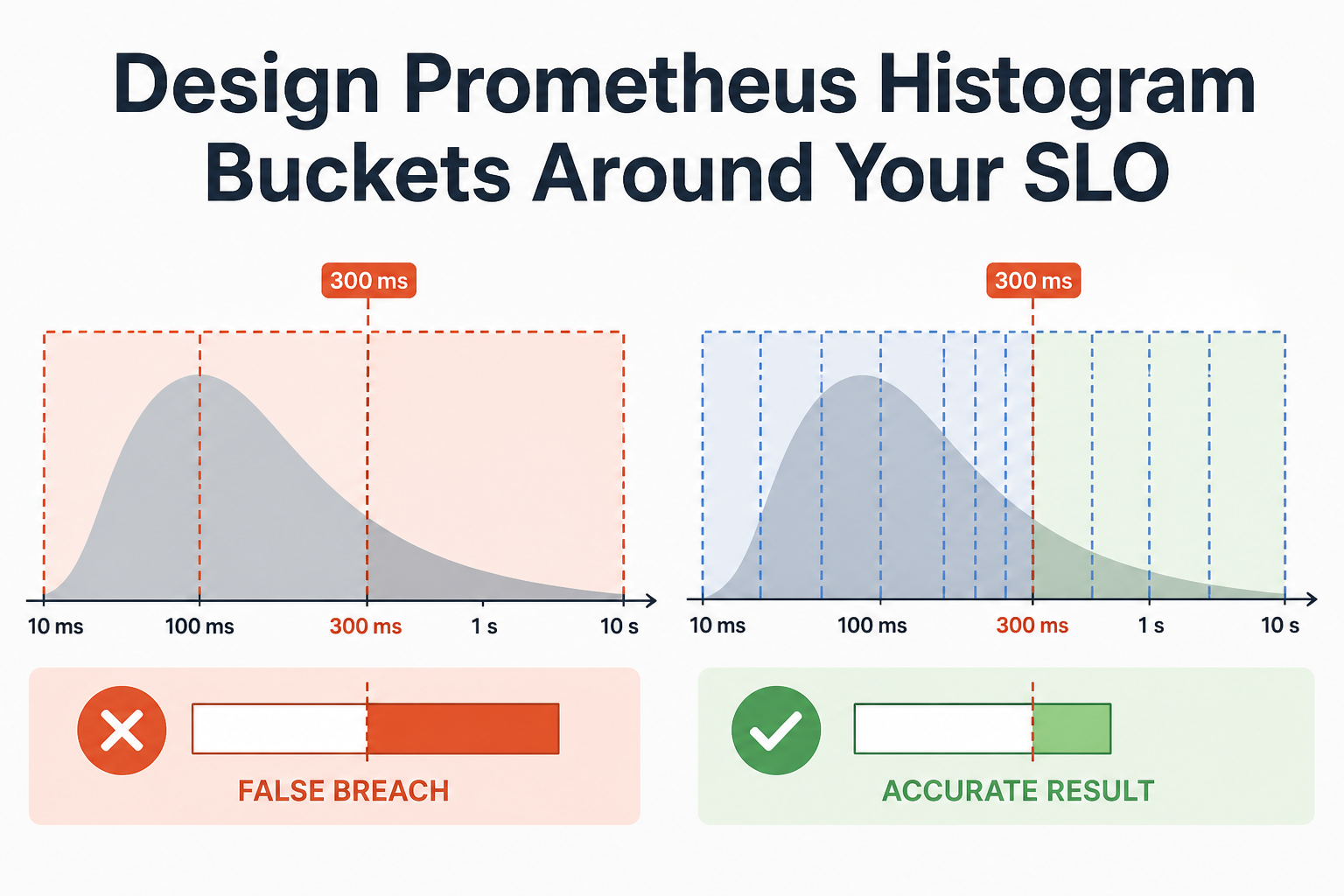
A Prometheus p95 alert can cross a 300 ms service-level objective even when the exact 95th observation is 290 ms. The alert may be mathematically consistent and operationally misleading: histogram_quantile() only knows cumulative bucket counts, so it estimates where the requested rank sits inside a bucket. A wide bucket can move the estimate across the SLO.
This guide proves that failure with Prometheus promtool rather than a conceptual chart. One fixed 100-request distribution is encoded twice as a classic histogram. The coarse layout estimates p95 at 0.50 seconds and reports a breach. A layout with boundaries near the decision estimates 0.30 seconds and preserves an exact 95% <= 0.30 threshold count. The extra precision also creates more time series, so the result ends with a cost and migration decision—not “add buckets everywhere.”
Developers and SREs maintaining classic Prometheus histograms can run the lab with Bash and Python 3 on Linux. It downloads an official checksum-verified Prometheus 3.13.2 archive into a marker-guarded /tmp path. It does not alter a service, scrape target, Prometheus server, dashboard, alert, or production metric.
The Bucket Layout Can Change the SLO Answer
Classic histograms publish cumulative counters such as http_request_duration_seconds_bucket{le="0.3"}. That series counts every observation less than or equal to 300 ms. Prometheus also publishes the implicit +Inf bucket, _sum, and _count. The current Prometheus histogram guidance explains that each classic bucket is a separate time series and that a threshold fraction is exact only when the layout contains that threshold.
histogram_quantile(0.95, ...) asks a different question. It finds the bucket containing rank 95 and interpolates within that bucket. The official PromQL function reference defines the aggregation and interpolation behavior. With classic histograms, retain le in the aggregation; dropping it destroys the cumulative layout the function needs.
For the controlled comparison, use this distribution:
| Latency | Request count | Cumulative share |
|---|---|---|
| 0.20 s | 90 | 90% |
| 0.29 s | 5 | 95% |
| 0.90 s | 5 | 100% |
Nearest-rank calculation puts p95 at 0.29 seconds. The coarse explicit boundaries are 0.10, 0.50, and 1.00; rank 95 lands at the top of the broad 0.10–0.50 bucket, so interpolation returns 0.50. The focused layout adds 0.25 and the SLO boundary 0.30; rank 95 then returns 0.30. This fixture is deliberately lumpy because production latency often clusters around cache paths, application paths, and timeouts rather than filling buckets uniformly.
Robust Perception’s histogram explanation is useful for cumulative-counter and aggregation mechanics. LinuxCzar’s quantile-error analysis examines the risk of assuming a uniform distribution inside a bucket. Neither source makes the synthetic distribution evidence about your workload; production boundaries must come from production observations and actual SLO decisions.
Pin the Disposable Prometheus Tooling
Run all blocks in one Bash shell so LAB and MARKER remain defined. The first block refuses to reuse an existing directory, pins the release version, verifies the archive against the release checksum file, and extracts only promtool.
set -Eeuo pipefail
LAB=/tmp/voxfor-prom-histogram-lab
MARKER="$LAB/.voxfor-prom-histogram-lab"
VERSION=3.13.2
ARCHIVE="prometheus-${VERSION}.linux-amd64.tar.gz"
BASE_URL="https://github.com/prometheus/prometheus/releases/download/v${VERSION}"

test ! -e "$LAB"
install -d -m 700 "$LAB/download" "$LAB/bin" "$LAB/evidence"
printf '%s\n' voxfor-prometheus-histogram-lab-v1 > "$MARKER"
curl -fsSL "$BASE_URL/sha256sums.txt" -o "$LAB/download/sha256sums.txt"
curl -fsSL "$BASE_URL/$ARCHIVE" -o "$LAB/download/$ARCHIVE"
(
  cd "$LAB/download"
  expected="$(awk -v file="$ARCHIVE" '$2 == file { print $1 }' sha256sums.txt)"
  test "${#expected}" -eq 64
  printf '%s  %s\n' "$expected" "$ARCHIVE" | sha256sum --check
)
tar -xzf "$LAB/download/$ARCHIVE" -C "$LAB/bin" --strip-components=1 \
  "prometheus-${VERSION}.linux-amd64/promtool"
"$LAB/bin/promtool" --version | tee "$LAB/evidence/promtool-version.txt"
On this run, the binary identified itself as promtool 3.13.2, revision bb5dff00cf8fdfbf5c65e0531aa835fa238a43a2, built with Go 1.26.5 for linux/amd64. Pinning the fixture separates a later PromQL semantic change from a bucket-layout change. In a real repository, pin the supported version for your deployment and update it through review.
Freeze One Distribution, Not Two Convenient Examples
Both layouts must derive from the same observations. The generator below records the raw grouped distribution, explicit boundaries, and cumulative counts. It also constructs a promtool test rules file with six counter samples from minute zero through minute five. Each minute adds the same 100 observations, which makes five-minute rate() ratios deterministic.
python3 - "$LAB" <<'PY'
import json, pathlib, sys

lab = pathlib.Path(sys.argv[1])
latencies = [0.20] * 90 + [0.29] * 5 + [0.90] * 5
layouts = {
    "coarse": [0.10, 0.50, 1.00],
    "focused": [0.10, 0.25, 0.30, 0.50, 1.00],
}

def cumulative(bounds):
    return {str(bound): sum(value <= bound for value in latencies) for bound in bounds}

fixture = {
    "unit": "seconds",
    "slo_seconds": 0.30,
    "quantile": 0.95,
    "observations": len(latencies),
    "distribution": [
        {"value_seconds": 0.20, "count": 90},
        {"value_seconds": 0.29, "count": 5},
        {"value_seconds": 0.90, "count": 5},
    ],
    "layouts": {
        name: {"explicit_bounds": bounds, "cumulative_counts": cumulative(bounds)}
        for name, bounds in layouts.items()
    },
}
(lab / "fixture.json").write_text(json.dumps(fixture, indent=2) + "\n")

series = []
for scenario, bounds in layouts.items():
    counts = cumulative(bounds)
    for bound in bounds:
        metric = f'http_request_duration_seconds_bucket{{scenario="{scenario}",le="{bound:g}"}}'
        series.append((metric, counts[str(bound)]))
    series.append((f'http_request_duration_seconds_bucket{{scenario="{scenario}",le="+Inf"}}', 100))
    series.append((f'http_request_duration_seconds_count{{scenario="{scenario}"}}', 100))

lines = [
    "rule_files: []", "evaluation_interval: 1m", "tests:",
    "  - name: classic histogram SLO layout", "    interval: 1m", "    input_series:",
]
for metric, increment in series:
    lines += [f"      - series: '{metric}'", f"        values: '0+{increment}x5'"]
lines += [
    "    promql_expr_test:",
    "      - expr: histogram_quantile(0.95, sum by (le, scenario) (rate(http_request_duration_seconds_bucket[5m])))",
    "        eval_time: 5m", "        exp_samples:",
    "          - labels: '{scenario=\"coarse\"}'", "            value: 0.5",
    "          - labels: '{scenario=\"focused\"}'", "            value: 0.3",
    "      - expr: histogram_quantile(0.95, sum by (le, scenario) (rate(http_request_duration_seconds_bucket[5m]))) > bool 0.3",
    "        eval_time: 5m", "        exp_samples:",
    "          - labels: '{scenario=\"coarse\"}'", "            value: 1",
    "          - labels: '{scenario=\"focused\"}'", "            value: 0",
    "      - expr: sum by (scenario) (rate(http_request_duration_seconds_bucket{le=\"0.3\"}[5m])) / sum by (scenario) (rate(http_request_duration_seconds_count[5m]))",
    "        eval_time: 5m", "        exp_samples:",
    "          - labels: '{scenario=\"focused\"}'", "            value: 0.95",
]
(lab / "histogram.test.yml").write_text("\n".join(lines) + "\n")
print(json.dumps({"observations": 100, "coarse_buckets": 3, "focused_buckets": 5}))
PY
Here, the scenario label exists only to compare layouts in one test. Do not deploy parallel metric layouts under a permanent unbounded experiment label. Use a temporary metric name or a bounded version label during migration, then retire it after the observation window.
Make PromQL Prove the SLO Classification
Next, the rule test executes three central claims against the real PromQL engine: p95 is 0.50 versus 0.30; the strict > 0.30 breach comparison is true only for the coarse layout; and an exact classic threshold fraction exists only for the focused layout.
"$LAB/bin/promtool" test rules "$LAB/histogram.test.yml" \
  | tee "$LAB/evidence/promtool-test.txt"
grep -q 'SUCCESS' "$LAB/evidence/promtool-test.txt"
promtool returned SUCCESS. The test is more useful than copying a dashboard number because it fixes the series, evaluation time, range window, query, expected labels, and values in a reviewable artifact. SigNoz’s explanation of rate() with histogram_quantile() reinforces the correct order: take rates over bucket counters, aggregate compatible buckets while retaining le, then calculate the quantile.
Do not aggregate classic histograms with different layouts under the same logical metric during a migration and assume the result remains interpretable. Keep old and candidate layouts distinguishable until the new series have a complete query window and the acceptance comparison is finished.
Require the Exact Threshold When Counting SLO Success
For the statement “95% of requests complete within 300 ms,” a classic histogram can calculate the direct fraction rate(bucket{le="0.3"}) / rate(count) only if 0.3 is an explicit boundary. Unlike histogram_quantile(), this classic query does not invent a missing threshold bucket by interpolation.
One boundary control fails the coarse layout with exit 3 and accepts the focused layout with the observed fraction 0.95. The same checker performs both decisions; the failure is not split into filler commands.
cat > "$LAB/check_boundary.py" <<'PY'
import json, sys
fixture = json.load(open(sys.argv[1]))
scenario = sys.argv[2]
layout = fixture["layouts"].get(scenario)
if layout is None:
    print(f"UNKNOWN_LAYOUT scenario={scenario}", file=sys.stderr)
    raise SystemExit(2)
slo = fixture["slo_seconds"]
if slo not in layout["explicit_bounds"]:
    print(f"MISSING_SLO_BOUNDARY scenario={scenario} slo_seconds={slo}", file=sys.stderr)
    raise SystemExit(3)
count = layout["cumulative_counts"][str(slo)]
print(f"SLO_BOUNDARY_OK scenario={scenario} le={slo} fraction={count / fixture['observations']:.2f}")
PY

set +e
python3 "$LAB/check_boundary.py" "$LAB/fixture.json" coarse \
  2>&1 | tee "$LAB/evidence/coarse-boundary-negative.txt"
coarse_rc=${PIPESTATUS[0]}
set -e
test "$coarse_rc" -eq 3
python3 "$LAB/check_boundary.py" "$LAB/fixture.json" focused \
  | tee "$LAB/evidence/focused-boundary.txt"
Expected outputs are MISSING_SLO_BOUNDARY scenario=coarse slo_seconds=0.3 and SLO_BOUNDARY_OK scenario=focused le=0.3 fraction=0.95. This gate protects the direct SLO fraction. It does not claim that a single five-minute window is a production SLO compliance period; choose alert and reporting windows from the actual SLO and error-budget policy.
Price the Added Resolution Before Instrumenting It
Every explicit classic boundary creates one _bucket series per label combination. The implicit +Inf bucket, _sum, and _count add three more. A three-boundary layout therefore produces six series per label set; five boundaries produce eight.
A separate receipt calculator derives the exact nearest-rank p95 from raw observations, reproduces Prometheus-style linear interpolation, and applies a concrete label budget: 12 routes × 3 methods × 2 regions × 4 replicas = 288 combinations.
python3 - "$LAB/fixture.json" <<'PY' | tee "$LAB/evidence/observed-receipt.txt"
import json, math, sys
fixture = json.load(open(sys.argv[1]))
q, total = fixture["quantile"], fixture["observations"]
values = []
for row in fixture["distribution"]:
    values.extend([row["value_seconds"]] * row["count"])
exact = sorted(values)[math.ceil(q * total) - 1]

def estimate(layout):
    bounds = layout["explicit_bounds"] + [math.inf]
    counts = [layout["cumulative_counts"].get(str(bound), total) for bound in bounds]
    rank, lower_bound, lower_count = q * total, 0.0, 0
    for upper_bound, upper_count in zip(bounds, counts):
        if upper_count >= rank:
            if math.isinf(upper_bound):
                return lower_bound
            return lower_bound + (upper_bound - lower_bound) * (rank - lower_count) / (upper_count - lower_count)
        lower_bound, lower_count = upper_bound, upper_count

combinations = 12 * 3 * 2 * 4
print(f"observations={total} exact_p95_seconds={exact:.2f} slo_seconds={fixture['slo_seconds']:.2f}")
for name, layout in fixture["layouts"].items():
    value = estimate(layout)
    series_per_set = len(layout["explicit_bounds"]) + 3
    status = "BREACH" if value > fixture["slo_seconds"] else "MEETS"
    boundary = fixture["slo_seconds"] in layout["explicit_bounds"]
    print(f"layout={name} estimated_p95_seconds={value:.2f} absolute_error_seconds={abs(value-exact):.2f} status={status} slo_boundary={str(boundary).lower()} series_per_label_set={series_per_set} projected_series={series_per_set*combinations}")
print(f"label_combinations={combinations} added_focused_series={(5-3)*combinations}")
PY
observations=100 exact_p95_seconds=0.29 slo_seconds=0.30
layout=coarse estimated_p95_seconds=0.50 absolute_error_seconds=0.21 status=BREACH slo_boundary=false series_per_label_set=6 projected_series=1728
layout=focused estimated_p95_seconds=0.30 absolute_error_seconds=0.01 status=MEETS slo_boundary=true series_per_label_set=8 projected_series=2304
label_combinations=288 added_focused_series=576
promtool=SUCCESS coarse_boundary_exit=3 focused_fraction=0.95Adding the focused layout spends 576 additional series in this label model. That may be reasonable for a service-level histogram and excessive for a metric labeled by raw path, tenant, customer, or request ID. Voxfor’s Prometheus label-cardinality diagnosis shows how label combinations multiply before bucket count is considered. Last9’s histogram bucket guide also emphasizes balancing useful resolution against resource cost.
Acceptance requires the official archive checksum to pass; promtool 3.13.2 to return SUCCESS; the same 100 observations to produce exact p95 0.29; the coarse layout to estimate 0.50, lack le="0.3", exit 3, and report a false breach; the focused layout to estimate 0.30 with 0.01-second absolute error and an exact threshold fraction of 0.95; and the declared 288 label combinations to produce 1,728 versus 2,304 series. If any identity, count, boundary, query, window, version, or label budget changes, generate a new receipt rather than reusing this verdict.
Migrate the Layout Without Erasing the Baseline
Changing classic boundaries in application instrumentation creates different time series and may leave queries spanning old and new layouts. Treat it as a metric migration:
- Inventory every producer, metric name, unit, label key, explicit boundary, recording rule, alert, dashboard, and remote-write consumer.
- Export a representative latency distribution by route or service class without high-cardinality request identities, then model candidate boundaries around real decision thresholds and meaningful tails.
- Emit the candidate under a temporary versioned metric name while the existing metric remains authoritative. Keep label keys and units consistent.
- Wait for at least the longest rate, recording-rule, alert, dashboard, and SLO reporting window before comparing old quantiles, exact threshold fractions, ingestion rate, active series, query latency, and alert state.
- Promote only when the candidate passes technical and cost criteria. Update recording rules before dashboards so one reviewed contract supplies downstream consumers.
- Keep the old metric through the rollback window. If ingestion or query cost breaches its budget, a required consumer has no candidate series, cumulative counts are invalid, or SLO classification is unstable, restore the old rules and instrumentation path.
Alert semantics deserve a separate decision. A valid p95 value can still be absent, stale, or replaced by an evaluation error. The Grafana No Data and Error policy guide explains why those states should not be collapsed into the latency threshold itself. End-to-end endpoint reachability is another layer; Prometheus Blackbox Exporter probes cover HTTP, DNS, and TLS evidence outside application latency instrumentation.
Latency SLOs also do not prove that a complete user path works. A separate customer-journey uptime test can validate the sequence a visitor needs, while the histogram explains the latency distribution inside the instrumented service. Keep these signals separate so a fast failing response does not look healthy and a slow but successful path does not disappear into availability alone.
Know When Native Histograms Change the Decision
Current Prometheus guidance prefers native histograms when the instrumentation library, exposition path, Prometheus version, remote-write backend, query consumers, and operational tooling support them. Native histograms store a histogram sample as one time series with a dynamic exponential schema, so the design knob becomes resolution and bucket limits rather than a permanent list of classic boundaries.
That does not make migration automatic. Confirm client-library support, scrape protocol, feature maturity, backend compatibility, recording rules, dashboard queries, alert behavior, storage, and rollback. The official practice page also describes ingesting classic histograms as native histograms with custom boundaries, with reconciliation caveats when layouts differ.
Use classic boundaries when you are maintaining existing classic metrics, need exact direct counts at contractual thresholds, or lack end-to-end native support. Evaluate native histograms when flexible quantiles, broader range, and more efficient resolution outweigh compatibility work. OneUptime’s current bucket-design overview provides additional implementation examples, but your acceptance evidence should come from your supported versions and observed distribution.
Metric ingestion is only one resource path. If an observability pipeline buffers data during a backend outage, the OpenTelemetry Collector memory and queue workflow helps separate histogram design from exporter backlog and process-memory risk.
FAQ: Prometheus Histogram Bucket Decisions
Should a Prometheus histogram include the exact SLO threshold?
For a classic histogram, include the threshold when you need an exact direct fraction such as requests at or below 300 ms. histogram_quantile() can still estimate a percentile without that boundary, but a wide surrounding bucket can move the estimate across the decision. Native histograms use a different resolution model and may interpolate the threshold.
Why can histogram_quantile report a false SLO breach?
It estimates the requested rank inside the bucket that contains it. If observations cluster near one edge while the bucket is wide, the interpolation assumption can overstate or understate the observed value. The function is behaving as designed; the layout lacks the resolution required for that decision.
Are more Prometheus buckets always better?
No. More classic buckets increase resolution and create more series for every label combination. Add boundaries where a measured distribution and reader decision require them, remove unused resolution deliberately, and calculate the full label multiplier before deployment.
Is p95 below 300 ms equivalent to 95% below 300 ms?
They are closely related but not interchangeable in every estimated histogram result. An exact nearest-rank p95 at or below 300 ms implies the raw distribution meets that threshold. A classic histogram quantile is interpolated; the direct le="0.3" bucket fraction is exact for the histogram counts when that boundary exists.
Can classic histograms with different boundaries be aggregated?
Do not assume they can be mixed safely under one logical query. A classic quantile needs compatible cumulative le series, and direct threshold queries omit producers without that boundary. Keep candidate and old layouts distinguishable during migration and compare complete windows before promotion.
Should a new service use native histograms instead?
Prefer evaluating native histograms when the entire collection, storage, remote-write, query, dashboard, and alert path supports them. They reduce fixed-boundary planning and can provide efficient resolution, but compatibility, resolution, bucket limits, query semantics, cost, and rollback still need testing.
Preserve the Receipt, Then Remove Only the Lab
Keep the production design record: metric and unit; producer versions; old and candidate boundaries or native resolution; measured distribution window; SLO thresholds; exact and estimated query results; label budget; projected and observed series; ingestion and query cost; downstream consumer inventory; comparison dates; acceptance owner; and rollback deadline.
Remove only the disposable fixture after verifying the exact path and marker:
test "$LAB" = /tmp/voxfor-prom-histogram-lab
test -f "$MARKER"
test "$(<"$MARKER")" = voxfor-prometheus-histogram-lab-v1
rm -rf --one-file-system "$LAB"
test ! -e "$LAB"
printf 'CLEANUP_OK path=%s absent=true\n' "$LAB"
This cleanup boundary applies only to the synthetic /tmp lab. A production rollback must keep the candidate evidence, restore the last accepted instrumentation and recording rules through the deployment system, wait for a complete query window, and verify old-series ingestion, SLO classification, alerts, dashboards, and active-series cost. Do not delete Prometheus data or change a live metric name merely to hide a failed candidate.