 Lifetime VPS Europe
 Lifetime VPS Asia
 Lifetime WooCommerce Hosting
 Lifetime Hosting
 Lifetime Game Dedicated Servers
 Chicago, US
 Tokyo, Japan
 Singapore
 Hong Kong
 Seoul, South Korea
 Amsterdem, Netherlands
 London, UK
 Stockholm, Sweden
 Oslo, Norway
 Vienna, Austria
 Zurich, Switzerland
 Sydney, Australia
 Wordpress Hosting
 VPS Hosting
 DDOS Protection
 Submit Ticket
 Full Management
 Guides
 Videos and Podcasts
 Discover Creative Ideas
 Voxfor Autonomous AI Workers
 Voxfor Mega Menu
 Voxfor Advanced Price Management For WooCommerce
 Voxfor Secure Live Chat and AI Support
 Voxfor Multilanguage
 Voxfor AI Content Summary
 Voxfor Autopilot
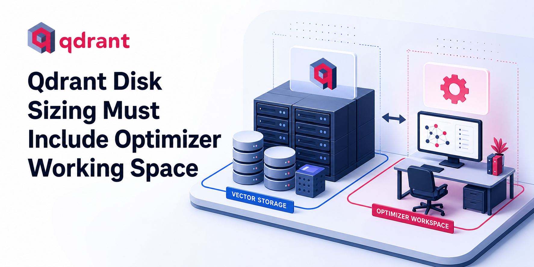
Raw vector bytes are only the first line in a Qdrant storage budget. A collection also carries payload, payload indexes, vector indexes, write-ahead records, segment metadata and point versions. During optimization, readable source segments can coexist with rebuilt segments and concurrent changes. A disk plan that ends at points × dimensions × 4 can therefore run out of space during normal maintenance even though the vectors appeared to fit.
Start with an estimate, but make the purchase decision from a representative ingest. For one million 1,024-dimensional float32 vectors, raw vector data begins near 4.10 GB decimal (1,000,000 × 1,024 × 4). Qdrant’s current capacity guidance applies a rough 1.5 estimation factor before payload, replicas and special recovery workspace, bringing that vector line to about 6.14 GB. That is a planning input, not a promise about final filesystem use.
Begin with the collection’s actual data model
Capacity belongs to the collection schema, not to a generic “vector database” label. Record expected point count, vector names, dimension and datatype for each vector, average and upper-percentile payload size, indexed payload fields, shard count, replica count, update rate and retention behavior.
Voxfor’s private vector-database deployment guide explains the wider RAG architecture. This worksheet starts one level lower: the bytes Qdrant must keep and rebuild after that architecture chooses Qdrant.
Count every vector attached to a point
A dense float32 vector uses four bytes per dimension before index and storage overhead. One 1,024-dimensional vector is 4,096 raw bytes. Named vectors add separate vector fields, while multivectors can attach several vectors to one point; point count alone no longer describes their size.
Use a separate line for each vector configuration:
raw vector bytes = points × vectors per point × dimensions × bytes per elementQuantization may reduce an in-memory or on-disk working representation, but do not subtract savings until a representative collection proves its actual segment size and search quality. Keep original-vector storage, index settings and rescore behavior visible in the test.
Sample payload instead of guessing from one JSON document
Payload varies much more than dimension. Sample serialized payload from real or production-shaped records, including keys, arrays and long-tail documents. Record at least an average and a high percentile, then identify which fields will receive payload indexes.
Current capacity planning guidance offers a rough payload estimate of points × payload size × 1.5. Its multiplier accounts for metadata, indexes, point versions and temporary segments, but the documentation also says to test with representative data. Treat 1.5 as an early sizing aid rather than guaranteed free-space policy.
Turn each storage component into a budget line
Keep logical data, physical placement and uncertainty in separate columns. Otherwise an on_disk choice can be mistaken for a reduction in total bytes when it primarily changes which layer serves them.
| Capacity line | Initial measurement | Placement question | Why the estimate can move |
|---|---|---|---|
| Dense vectors | points × dimension × datatype bytes | RAM or mmap/on-disk | named vectors, multivectors and quantization |
| Payload | representative serialized sample × points | RAM or on disk | document distribution and updates |
| Payload indexes | only fields needed for filters | indexed values remain performance-sensitive | field types and cardinality |
| Vector index | build with intended HNSW settings | HNSW in RAM or on disk | graph parameters and segment shape |
| Segment/WAL overhead | measure after representative ingest | same fast local storage in most deployments | point versions, deletes and update rate |
| Working space | observe an optimizer cycle | unallocated on the data filesystem | merge concurrency and segment sizes |
Storage documentation describes segments as self-contained units with vector storage, payload storage, vector and payload indexes, and an ID mapper. WAL protects changes before they are incorporated into segments. These are functional parts of the database, not optional “miscellaneous” bytes.
Replicas multiply placement, not vector dimensions
Calculate a per-replica collection budget first. Then map each replica to a peer and filesystem. A replication factor of two normally means two physical copies across the cluster, but it does not mean every node necessarily holds both copies. Per-node capacity depends on shard placement; cluster capacity depends on all replicas plus failure and rebalance policy.
Keep embedding generation outside this arithmetic. GPU infrastructure choices for AI workloads may change where embeddings are computed, but a remote GPU does not remove Qdrant’s vector, index or payload storage.
Optimizer working space changes the safe floor
During optimization, Qdrant does not rewrite a live segment in place and make it unavailable until completion. Its optimizer documentation explains that a source segment remains readable while an optimized segment is built. Concurrent updates go into a copy-on-write segment and are applied to the rebuilt result. Merge optimization can also create temporary segments while combining smaller segments.
That behavior protects availability, yet it means old and new representations may overlap. Peak use depends on which segments qualify, their size, concurrent optimizer jobs and writes arriving during the rebuild. A universal “leave 20% free” rule is not supported by those variables.
Measure ordinary overlap separately from recovery space
Create two headroom records:
- Operating workspace: the observed filesystem peak during representative ingest, indexing, deletes and an optimizer cycle, plus an explicit growth interval and uncertainty margin chosen by the operator.
- Special-operation workspace: additional target capacity required by a planned migration, snapshot recovery or rebalance procedure.
For special operations, capacity guidance says a Migration Tool target should have twice the source collection’s disk space, and snapshot recovery into a new deployment similarly needs target disk equal to twice the collection size. Do not apply that statement silently as a universal steady-state multiplier; attach it to the operation that needs it.
Snapshots should not depend on the same nearly full data volume for both source and recovery copy. They are recovery artifacts, not optimizer workspace. An AI application operator following Voxfor’s AI agent VPS workspace guidance should keep application state, credentials and vector-database recovery ownership explicit rather than treating one server disk as an undifferentiated pool.
Replace estimates with a representative ingest
Build a test collection with the intended vector configuration, payload indexes, shard count and on-disk settings. Load enough production-shaped points to create multiple realistic segments; a tiny sample that remains in one segment will not expose the same index and optimizer behavior.
Resolve the deployed data directory before measuring it. A native/service installation can set storage.storage_path in Qdrant configuration, so do not assume one filesystem path. The official local Docker quickstart mounts host directory ./qdrant_storage to container directory /qdrant/storage. Measure the host mount when planning host capacity, or the configured data path when Qdrant runs directly.
Replace the placeholder below with that deployed directory, then record bytes and free space before ingest:
QDRANT_DATA_DIR=/path/to/deployed/qdrant/storage
date -u; df -B1 "$QDRANT_DATA_DIR"; du -sx --block-size=1 "$QDRANT_DATA_DIR"
Query collection state without printing payload content:
curl -fsS "http://127.0.0.1:6333/collections/${COLLECTION}" | jq '{status: .result.status, points: .result.points_count, vectors: .result.vectors_count, segments: .result.segments_count, optimizer: .result.optimizer_status}'Use a local authenticated or network-isolated endpoint appropriate to the deployment. Do not put an API key directly in shell history. If the endpoint requires a credential, load it from the deployment’s protected secret mechanism and redact command output before attaching it to a ticket.
Capture a peak, not one quiet snapshot
Repeat byte measurements while ingestion, index creation and optimization are active. Current Qdrant monitoring exposes collection, vector, optimizer and I/O signals through /metrics; monitoring documentation recommends scraping each peer separately.
curl -fsS http://127.0.0.1:6333/metrics | grep -E 'collection_(points|vectors|running_optimizations)|vector_io|payload_io'Metric names can vary with Qdrant version, so inspect the endpoint actually deployed instead of hard-coding an alert from this example. Bound collection and peer labels deliberately. Voxfor’s Prometheus label-cardinality workflow shows why an unbounded label can turn a useful storage alert into its own resource problem.
Record four checkpoints: empty collection, completed ingest, active optimizer peak and settled post-optimization state. Divide observed settled bytes by loaded points, compare the ratio with the initial vector/payload estimates, and preserve both results. The difference is evidence, not an error to hide.
Decide which layer RAM or SSD will carry
Vectors can remain in memory or use Qdrant’s mmap/on-disk storage. HNSW indexes can also be placed on disk. Payload may move to disk, while indexed payload values remain important to filtering performance. Page cache means an on-disk configuration can still show high resident memory; on_disk: true is not a promise that RAM use approaches zero.
Optimization guidance recommends local SSD capable of at least 50,000 IOPS for on-disk search and warns that heavy updates make optimizers compete for CPU, memory and I/O. Treat that figure as a documented minimum direction, then benchmark the exact vector dimension, filter mix and latency objective on intended storage.
Choose placement in this order:
- Keep latency-critical vector or HNSW layers in RAM when the measured working set and failure policy fit.
- Move vectors or HNSW to mmap/on-disk when capacity is larger than practical RAM, then prove cold and warm query latency.
- Put payload on disk only after representative filters prove acceptable latency and required fields are indexed.
- Preserve SSD I/O runway for optimizer work, WAL and application queries at the same time.
Translate measured per-node requirements into an actual VPS hosting plan only after CPU, RAM, local SSD capacity and IOPS are all recorded. Disk size alone cannot validate an on-disk search design.
Release the capacity plan only after a growth test
A production-ready worksheet contains more than a final gigabyte number. Record collection schema, Qdrant version, point sample, settled bytes per point, active-optimizer peak, projected growth interval, replica placement, free-space alert floor and special-operation requirement. Repeat the test after a meaningful payload, index or quantization change.
Approve the plan when all of these statements are true:
- A representative collection reaches the expected point, vector and payload distribution.
- Query latency remains inside its objective during an optimizer cycle.
- Every peer preserves its recorded operating floor at the measured peak.
- Replica placement still fits after the planned node-failure or rebalance case.
- Migration or snapshot recovery has separately reserved target capacity and a tested procedure.
Continue through Voxfor’s AI and hosting library for adjacent deployment work, but keep this budget versioned with the collection. The useful result is not “Qdrant needs 30 GB.” It is a measured statement that explains which bytes exist, where they live, when they overlap and which operation owns the remaining free space.
FAQ: Qdrant storage capacity decisions
How much storage does one Qdrant vector need?
A dense float32 vector starts at dimension multiplied by four bytes. A 1,024-dimensional vector is 4,096 raw bytes, before vector indexes, segment metadata, payload, point versions, replicas and optimizer working space.
Why does Qdrant need disk beyond raw vector bytes?
Stored payload, indexes, ID mappings, WAL and segment metadata sit alongside Qdrant vectors. Optimization can temporarily keep readable source segments and rebuilt segments at the same time, while concurrent writes use copy-on-write handling.
Does on_disk: true remove Qdrant RAM requirements?
No. On-disk vectors or indexes use mmap and operating-system page cache, and indexed payload/filter structures still need memory. Measure resident memory and cold/warm query latency with the intended workload.
Should Qdrant snapshots share the live data volume?
Avoid making a nearly full data volume the only location for live segments and recovery artifacts. Snapshot storage, retention and restore targets should have explicit ownership and capacity separate from ordinary optimizer workspace.
How much headroom does Qdrant migration or snapshot recovery need?
Current Qdrant capacity guidance documents target disk equal to twice the source collection size for its Migration Tool and for snapshot recovery into a new deployment. Reserve that for the named operation and still validate the procedure with the deployed version and topology.